7  Radiomics Workflow

References: (Shur et al. 2021), (Timmeren et al. 2020)

7.1 Planning

7.1.1 Sample Size

• a radiomic signature (defined as the learned model from a radiomic analysis used to predict a particular clinical outcome)

• For binary classification studies: 10–15 samples per feature

  • Apply this rule to the smaller class if class sizes are unequal.

• Data attrition: Common due to:

  • Missing or mislabeled data.
  • Failure to meet inclusion criteria.
  • Loss to follow-up.
  • Poor image quality.

7.1.2 Validation

One-third of the training sample size (range of 60:40 to 90:10.)

• a trade-off between having enough data in the training set to ensure the model has sufficient predictive power and having a large- enough test dataset to ensure the predicted performance estimate is accurate

Example:

A 10-feature model, at least total 133 samples are required

• 100 are used for training
• 33 for validation.

If Assuming an attrition rate of 50% would require a total study population of 266.

7.1.3 Pilot Samples

• For classification studies, a pilot sample size of 12 per class has been proposed (Julious 2005), but in practice this is guided by available resources and the study population

7.1.4 Class balanced ?

• Balanced data: Each class or outcome contains an approximately equal proportion of data.

• Unbalanced data: Unequal class proportions.

  • If highly unbalanced, a larger sample size may be required for a generalizable model.

7.1.5 Heterogenitey

Trade-off in datasets:

• Heterogeneous datasets: Real-world data with potential noise, possibly masking the radiomic signature.
  • Less rigidly standardized protocols can be used to reflect real-world clinical scenarios.
• Homogeneous datasets: Less noisy, but lower generalizability.
  • Standardized imaging protocols (ie, those that use the same vendor or scanner settings for all samples) can be used to reduce unwarranted confounders and noise

7.2 Image Acquisition

7.2.1 Modalitis

Often determined by what is available and used in clinical practice.

• CT and PET data are that signal intensities (SIs) are inherently quantitative.

• MRI SI are arbitrary, and hence normalization of SI is recommended.

• US is more user dependent than other modalities.

• Contrast-enhanced imaging yields information about tumor enhancement, vascularity, and heterogeneity

7.2.2 Images

• Anonymized to remove patient identifiable metadata.

• Exported as Digital Imaging and Communication in Medicine (DICOM) files by using a lossless- compressed format

7.3 Segmentation

7.3.1 Regions

Segmentation can be performed by drawing ROIs on:

• The tumor
• Tumor subregions (“habitats”)
• Peritumoral zones

The choice guided by the research hypothesis.

7.3.2 ROI methods

ROIs can be delineated:

• Automatically:
  • Potentially faster and more reproducible
  • may be required for larger dataset
  • can be compared against those obtained after manual segmentation by using the Dice score.
  • Deep learning-based image segmentation
• Semiautomatically:
  • using standard image segmentation algorithms such as region-growing or thresholding
• Manually:
  • Feature stability should be assessed: performing multiple segmentations of the same tumor with either the same or a different reader performing the delineation.

in either two dimensions (2D) (single section) or three dimensions (3D) (multiple sections)

Drawbacks of manual and semi-automated image segmentation:

• Time-consuming: depending on how many images and datasets have to be segmented.
• Observer-bias
  • Many radiomic features are not robust against intra- and inter-observer variations concerning ROI/VOI delineation
  • should perform assessments of intra- and inter-observer reproducibility of the derived radiomic features and exclude non-reproducible features from further analyses.

7.4 Image Preprocessing

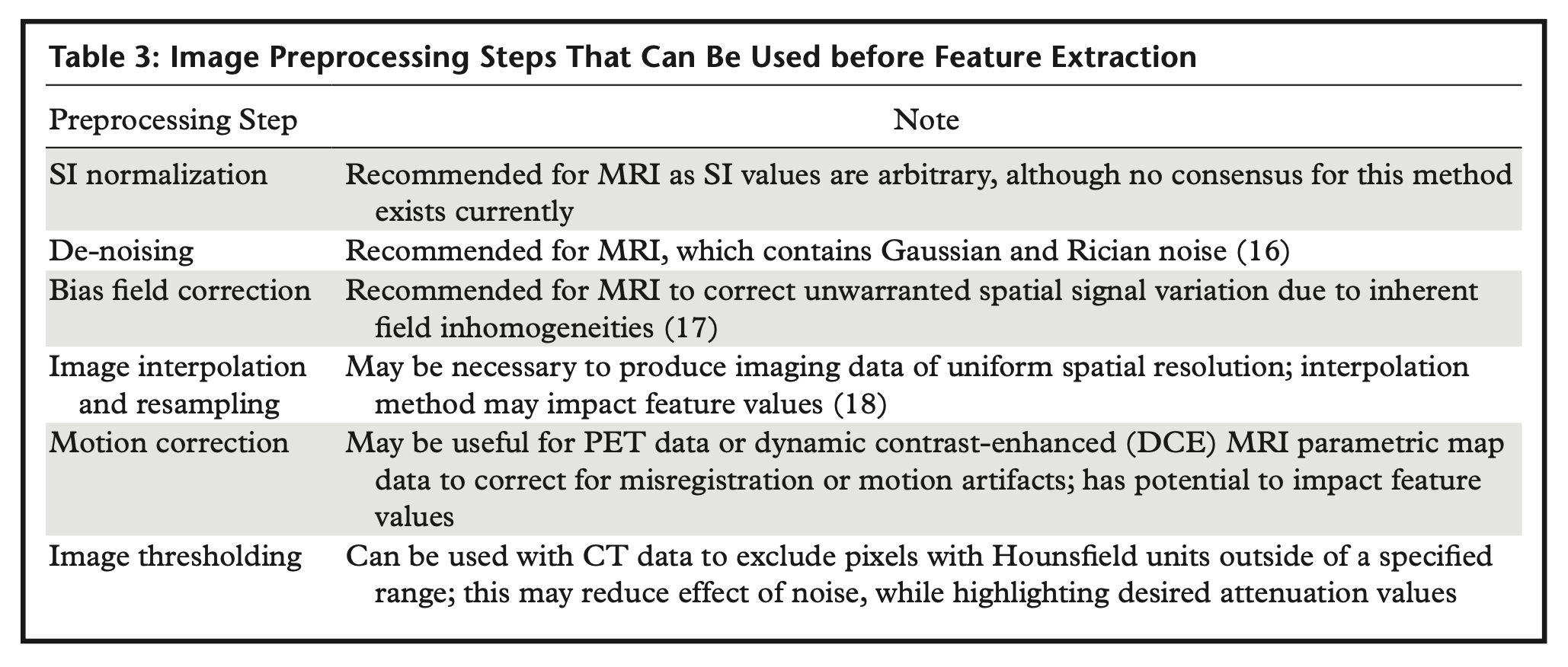
Raw image data can be enhanced through a variety of preprocessing steps:

Figure 7.1: Image Preprocessing (Shur et al. 2021)

7.4.1 Interpolation to isotropic voxel spacing

As some radiomic feature values are dependent on voxel size (Shafiq-Ul-Hassan et al. 2017), images should be resampled to a common spatial resolution for all samples.

• Linear interpolation is generally recommended

For most texture feature sets to become rotationally invariant and to increase reproducibility between different datasets (Timmeren et al. 2020).

• CT: usually delivers isotropic datasets

• MRI: often delivers non-isotropic data with need for different approaches to interpolation

7.4.2 Range re-segmentation and intensity outlier filtering (normalization)

Performed to remove pixels/voxels from the segmented region that fall outside of a specified range of grey-level (Timmeren et al. 2020).

• Range re-segmentation:

  • Required for CT and PET data (e.g., for excluding pixels/voxels of air or bone within a tumor ROI/VOI)
  • Same concept as Section 7.4.6.2

• intensity outlier filtering:

  • For MRI data
  • Most commonly used method: to calculate the mean (μ) and standard deviation (σ) of grey-levels within the ROI/VOI and to exclude greylevels outside the range μ ± 3σ

7.4.3 Discretization

last image processing step is discretization of image intensities inside the ROI/VOI. Discretization consists in grouping the original values according to specific range intervals (bins); the procedure is conceptually equivalent to the creation of a histogram (Timmeren et al. 2020).

7.4.3.1 Parameters characterize discretization:

• Range of the discretized quantity = Number of bins x Bin width
• Number of bins
• Bin width (size)

Different combinations can lead to different results; the choice of the three parameters is usually influenced by the context:

• The range is usually preserved from the original data, but exceptions are not uncommon, e.g. when the discretized data is to be compared with some reference dataset or when ROIs with much smaller range than the original have to be analyzed. It is worth mentioning that when the range is not preserved and if the number of bins is particularly small, the choice of the range boundaries can have a strong impact on the results

7.4.3.2 Fixing the bin number

• Fixing the bin number (as is the case of discretizing grey-level intensities) normalizes images and is especially beneficial in data with arbitrary intensity units (e.g., MRI) and where contrasts are considered important.
• The use of a fixed bin number discretization is thought to make radiomic features more reproducible across different samples

(controversies: Pyradiomics FAQ)

7.4.3.3 Fixing the bin size

• results in having direct control on the absolute range represented on each bin, therefore allowing the bin sequence to have an immediate relationship with the original intensity scale (such as Hounsfield units or standardized uptake values).
• This approach makes it possible to compare discretized data with different ranges, since the bins belonging to the overlapping range will represent the same data interval.
• For that reason, previous work recommends the use of a fixed bin size for PET images
• It is recommended to use identical minimum values for all samples, defined by the lower bound of the re-segmentation range

7.4.3.4 Open Question: optimal bin number/bin width

• Bins are too wide (too few): features can be averaged out and lost
• Bins are too small (too many): features can become indistinguishable from noise

A balance is reached when discretization can filter out the noise while preserving the interesting features

small number of bins can generate undesired dependencies on the particular choice of range and bin boundaries, thus undermining the robustness of the analysis.

different MRI sequences might need different bin numbers for obtaining robust and reproducible radiomics features (Wichtmann et al. 2023)

recommendation is to always start by inspecting the histogram of the data from which radiomic features are to be extracted and to decide upon a reasonable set of parameters for the discretization step based on the experience.

7.4.4 Motion correction

Motion correction can be used to correct for misregistration, blurring, or motion artifacts and has been used in four-dimensional CT of lung tumors

7.4.5 Image filtration

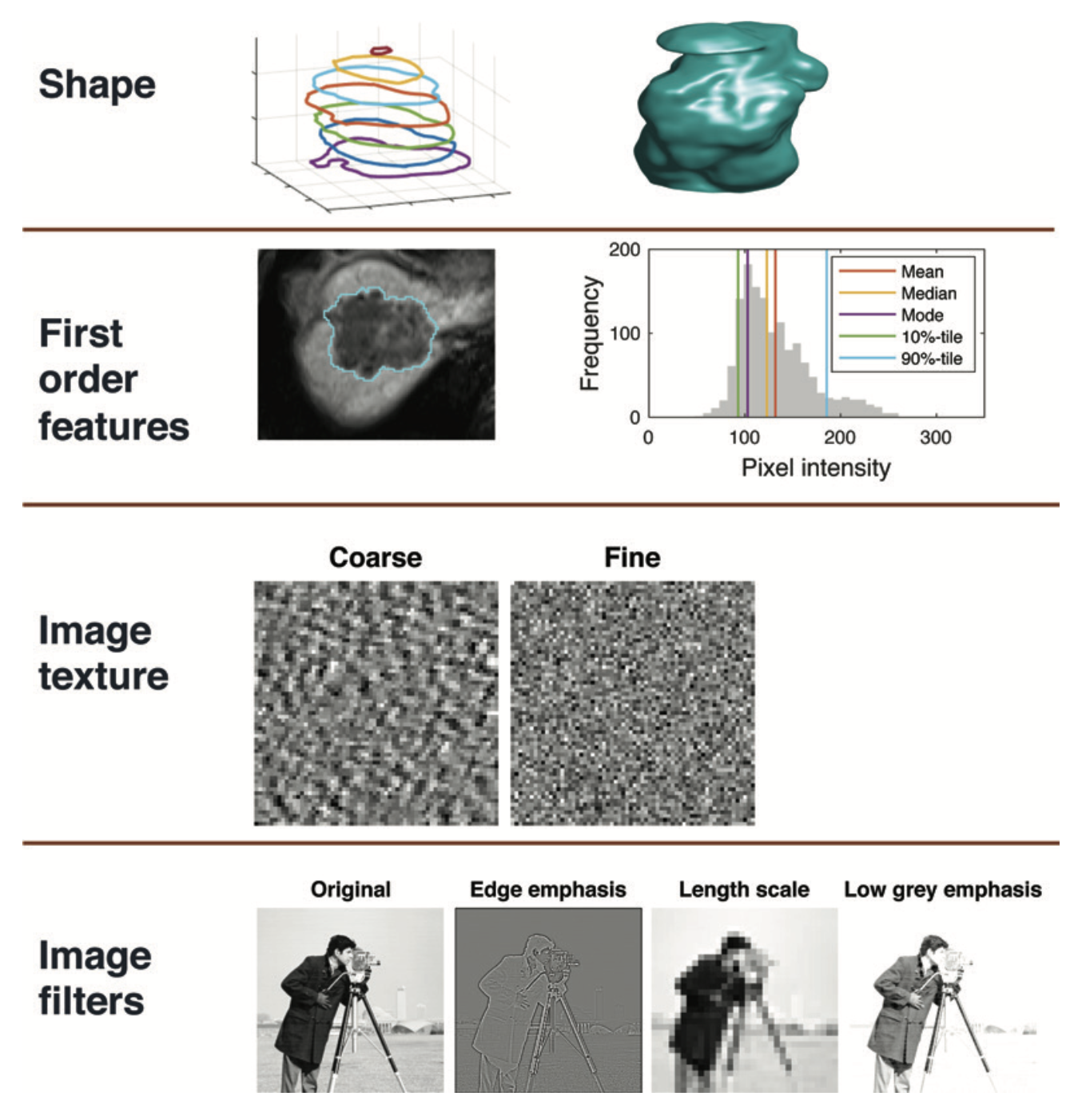
Image filtration can be used before the extraction of features as a preprocessing step to highlight particular image properties.

• Nonspatial filters increase or decrease the sensitivity of the radiomics features to high- or low-intensity values
  • Examples: taking the square or exponential of the image intensities
• Spatial filters increase or decrease the sensitivity of features to particular spatial properties of the image. Examples:
  • Laplacian of Gaussian (LoG) filters: emphasize areas of rapid change (eg, edge detection)
  • Wavelet filters: separate high- and low-spatial-frequency information.

number of radiomics features (and hence datasets) generated with image filtration can become large, so it is typical to try using unfiltered images first.

Figure 7.2: Image Feature & Filter (Shur et al. 2021)

7.4.6 Summary by Modalities

7.4.6.1 MRI Preprocessing

• Bias field correction should also be applied to correct for the spatial field inhomogeneities encountered with MRI
  • Note: done before segmentation
• Z-score normalization is a simple method and is computed by subtracting the mean SI of the region of interest (ROI) from the pixel SI and dividing the result by the standard deviation
  • Note: done after segmentation
• Fixing the bin number: normalizes images and is especially beneficial in data with arbitrary intensity units (e.g., MRI) and where contrasts are considered important

7.4.6.2 CT Preprocessing

• Thresholding on voxel Hounsfield units can be applied to CT data to exclude voxels that are assumed to contain noninformative tissues.
  • For example, very low values may correspond to air within the lung and high values to bone or calcification.

7.5 Feature Extraction

Standardization: Image Biomarker Standardization Initiative (IBSI)

7.5.1 Feature Classes

7.5.1.1 Morphologic

Morphologic features: describe geometric properties of the lesion such as volume, diameter, surface area, and elongation

7.5.1.2 First-Order (Intensity-based)

First-order features: (Intensity-based) describe properties of the distribution of intensities within an ROI, where the spatial location of each voxel is ignored:

• Location of the distribution: mean, median, mode, etc
• Spread of the distribution: variance, interquartile range, etc
• Shape of the distribution: skewness, kurtosis, etc (unaffected by image standardization)
• Voxel intensity heterogeneity (entropy, energy, etc)

MRI and US typically generate images with arbitrary intensity scaling, and if this is not consistent for all subjects it will be necessary to apply image standardization before calculating first-order features

7.5.1.3 Second-order (texture)

Second-order features: also known as texture features, go beyond first-order features so that the spatial locations as well as the SIs of two or more pixels are used when computing the features.

7.5.1.4 Intensity discretization

Intensity discretization involves assigning pixels within a given intensity range to a single value or “bin” and is used before calculation of secondorder features.

• Reducing the number of bins (or increasing the bin width) will lead to a loss of image detail but will remove noise

• Increasing the number of bins (or decreasing the bin width) will retain more image detail but will also preserve image noise

Note:

• When image intensity units are arbitrary (such as with MRI data), fixing the number of bins (rather than the bin size) is recommended
• Whichever method is used, it should be the same for all patients.

7.5.1.5 Semantic features

Semantic features such as “spiculated” or “enhancing” can also be used as input features to a radiomics model and will be determined by visual inspection.

These features will typically be categorical (eg, small, large, hy- perenhancing) rather than numerical.

7.6 Feature Selection

The higher the number of features/variables in a model and/or the lower the number of cases in the groups, e.g., for a classification task, the higher the risk of model overfitting. (Timmeren et al. 2020)

Steps:

1. Exclusion of non-reproducible features:
   • A feature which suffers from higher intra- or interobserver variability is not likely to be in- formative
   • Simply assessing reproducibility/robustness by calculation of intra-class- correlation coefficients (ICCs) might not be sufficient since ICCs are known to depend on the natural variance of the underlying data
   • Recommendations for assessing reproducibility, repeatability, and robustness
2. Selection of the most relevant variables:
   • ML based: knock-off filters, recursive feature elimination methods, or random forest algorithms
   • Correlation clusters -> selection of only one representative feature per correlation cluster.
     • The variable with the highest biological-clinical variability in the dataset should be selected since it might be most representative of the variations within the specific patient cohort.
3. Leaving -> non-correlated and highly relevant features

Julious, Steven A. 2005. “Sample Size of 12 Per Group Rule of Thumb for a Pilot Study.” Pharmaceutical Statistics 4 (4): 287–91. https://doi.org/10.1002/pst.185.

Shafiq-Ul-Hassan, Muhammad, Geoffrey G. Zhang, Kujtim Latifi, Ghanim Ullah, Dylan C. Hunt, Yoganand Balagurunathan, Mahmoud Abrahem Abdalah, et al. 2017. “Intrinsic Dependencies of CT Radiomic Features on Voxel Size and Number of Gray Levels.” Medical Physics 44 (3): 1050–62. https://doi.org/10.1002/mp.12123.

Shur, Joshua D., Simon J. Doran, Santosh Kumar, Derfel Ap Dafydd, Kate Downey, James P. B. O’Connor, Nikolaos Papanikolaou, Christina Messiou, Dow-Mu Koh, and Matthew R. Orton. 2021. “Radiomics in Oncology: A Practical Guide.” Radiographics: A Review Publication of the Radiological Society of North America, Inc 41 (6): 1717–32. https://doi.org/10.1148/rg.2021210037.

Timmeren, Janita E. van, Davide Cester, Stephanie Tanadini-Lang, Hatem Alkadhi, and Bettina Baessler. 2020. “Radiomics in Medical Imaging—‘How-to’ Guide and Critical Reflection.” Insights into Imaging 11 (1): 91. https://doi.org/10.1186/s13244-020-00887-2.

Wichtmann, Barbara D., Felix N. Harder, Kilian Weiss, Stefan O. Schönberg, Ulrike I. Attenberger, Hatem Alkadhi, Daniel Pinto Dos Santos, and Bettina Baeßler. 2023. “Influence of Image Processing on Radiomic Features from Magnetic Resonance Imaging.” Investigative Radiology 58 (3): 199–208. https://doi.org/10.1097/RLI.0000000000000921.